Sunday, January 31, 2010

Tesserae, sera

Fig3-14
Figure 3.14. A solute–solvent boundary surface described by a set of interlocking atom-centered spheres. The surface is discretized by using triangular tesserae. Drawing graciously provided by Benedetta Mennucci.
From Molecular Modeling Basics CRC Press, May 2010.

Due to the computational expense of explicit solvation, implicit solvation is a popular alternative when including solvent effects in quantum chemical calculations. The polarized continuum model (PCM) and the closely related COSMO method is one of the most used implicit solvation models for QM calculations. Here the Poisson-Boltzmann equation is solved numerically by diving the solute-solvent surface into small pieces called tesserae (Figure 3.14).

Unfortunately, I have not been able to make an interactive version of this figure.

Wednesday, January 27, 2010

It's all about boundaries

Fig3-8
Figure 3.8. (a) Adenine (C5H5N5) in a liquid drop of 246 water molecules. (b) Adenine in a periodic box of 511 water molecules.
From Molecular Modeling Basics CRC Press, May 2010.

Conceptually, the simplest way of simulating a molecule in solution is to place it in the middle of a roughly spherical ball of water molecules (Figure 3.8a) and perform an molecular dynamics simulation.

One problem is this approach is that the drop would eventually evaporate if the simulation is run long enough. Another problem with the liquid drop model is that the water molecules at the surface of the drop do not behave like water molecules in liquid water.

Therefore, most explicit solvation simulations use periodic boundary conditions (Figure 3.9).

Fig3-9
Figure 3.9. Sketch of periodic boundary in two dimensions: (a) The position of the particles in the central box are copied and placed in neighboring boxes. Figure 3.8b shows a cube from a real simulation. (b) When a molecule tries to leave the box during an MD simulation, it reappears at the opposite end of the box, so the number of particles in the central box stays constant.
From Molecular Modeling Basics CRC Press, May 2010.

You can find interactive versions of Figures 3.8a and 3.9b here (I am grateful to Kestutis Aidas for providing the coordinates).

Click on the picture for an interactive version

And you can find an animated version of Figure 3.9 here (an example of where a movie really is worth 10,000 words).


The animation was made with Molecular Workbench (MW). You can play with the simulation here or you can download the MW file here (after you gave installed MW).

Saturday, January 23, 2010

I have my moments

Fig3-7
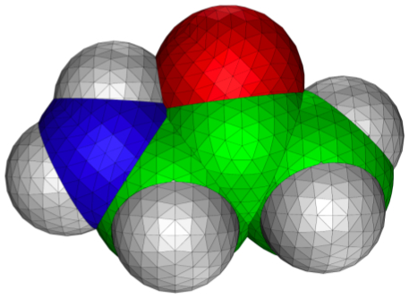
Figure 3.7. Contour plot of the RHF/6-31G(d) electrostatic potential and 0.002 au isodensity surface of (a) CH3COO-, (b) HF, and (c) F2. The maximum/minimum contour values are, respectively, 0.5/0.025; 0.1/0.005; and 0.005/0.00025 au respectively. Blue corresponds to a negative potential. In each case the outer-most contour looks like the corresponding contour in the electrostatic potential due to a charge, dipole, and quadrupole, respectively.
From Molecular Modeling Basics CRC Press, May 2010.

This figure makes 3 points:

1. It shows what the electrostatic potential of a charge, dipole, and quadrupole looks like.

2. It show the relative strengths of the electrostatic potentials due to a charge, dipole, and quadrupole.

3. It shows that the electrostatic potential of a charge, dipole, and quadrupole deviates significantly from the actual electrostatic potential near the molecular surface.

Here is a screencast showing how I made Figure 3.7a. (If I were to do it over I would have chosen red for negative and blue for positive... oh, well.)

Here is an interactive version of the figure. Click on the picture to load it. Remember it's Jmol so you can rotate it and zoom as you like (Mac users: this works best with Safari).
Figure 3.7. The RHF/6-31G(d) electrostatic potentials of acetate, HF and F2.
Click on the picture for an interactive version

See these two posts (here and here) on how to make plots like that with Jmol. From a Jmol perspective the only new thing is that I show two isosurfaces simulateneously. This is done by loading the file twice to create two "frames" that Jmol can display simultaneously. You can find the script file with all the commands here, but the general syntax is:

load files file1.xyz file2.xyz
frame 1.1; isosurface surf1 plane {0 0 0 0} contour 40 color range -0.05 0.05 "potential.cube.gz"
frame 2.1; isosurface surf2 0.002 "density.cube.gz" 
Even though you want a 2D contour plot of the potential, it is necessary to make a 3D cube file. Because I use unusually low cutoffs to show the outer contours, I had to trick MacMolPlt into making a bigger grid. I show how on the screencast below.

Saturday, January 2, 2010

Common error messages in GAMESS: Failure to locate stationary point

***** FAILURE TO LOCATE STATIONARY POINT, TOO MANY STEPS TAKEN *****
  UPDATED HESSIAN, GEOMETRY, AND VECTORS WILL BE PUNCHED FOR RESTART
**** THE GEOMETRY SEARCH IS NOT CONVERGED! ****
This error message was produced by the following input file. Can you see what's wrong?
$contrl runtyp=optimize icharg=1 $end
 $basis gbasis=pm3 $end
 $data
Title
C1
N     7.0    -0.39094     1.95659     0.14008
H     1.0     0.38874     1.60529    -0.40413
H     1.0    -0.08386     2.76975     0.70945
H     1.0    -0.72485     1.22934     0.80007
H     1.0    -1.14035     2.30329    -0.48754
O     8.0    -0.64579     0.16732     2.03360
H     1.0    -0.26212    -0.73042     2.10569
H     1.0    -1.00756     0.26750     2.93979
O     8.0    -1.80535     3.31298    -1.59619
H     1.0    -1.39440     3.81065    -2.33214
H     1.0    -2.74148     3.57968    -1.71559
O     8.0     0.26578     4.05264     1.54485
H     1.0     1.03270     4.27032     2.11226
H     1.0    -0.26135     4.87344     1.64760
 $end
Actually, there is no problem with the input file as such. A geometry optimization is an iterative process and if the gradient it not below the convergence criteria within 20 steps, GAMESS will stop and print out the message shown above.

The solution is simply to take the last set of coordinates and run the optimization again, as I show in the screencast below.

As I've mentioned in a previous post I think the default criterion for geometry convergence (0.0001) is too strict, and the default number of steps (20) is too small. So I usually use 0.0005 and 50, respectively.
$statpt nstep=50 opttol=0.0005 $end